Exploratory Data Analysis Best Practices for Exhaustive Data Analysis

Introduction

EDA, short for Exploratory Data Analysis, or as I like to call it, Data Reveal Party 😊 (because it’s fun playing around and getting your hands dirty with datasets) is one of the most important steps towards a successful data project. You get to uncover hidden data insights that only this process can unearth. It is therefore good practice to make sure you exhaust on it by investigating and looking at the dataset from every possible angle. In this article we are going to look at the steps to follow to accomplish this when doing EDA.

EDA Steps

1. General dataset statistics

Here you investigate the structure of your dataset before doing any visualizations. General dataset stats may include but are not limited to:

• small overview of dataset - head(), tail() or even sample()
• size and shape of dataset
• number of unique data types
• number of numerical and non-numerical columns
• number of missing values per column
• presence of duplicate values
• column names - correct naming of column names to one word for ease of calling columns from the dataframe object

This is just to familiarise yourself with the dataset. Let’s wrap all these steps in a single python function:

 1
 2
 3
 4
 5
 6
 7
 8
 9
10
11
12
13
14
15
16
17
18
19
20
21
22
23
24
25
26
27

# Necessary imports
import numpy as np
import pandas as pd
import matplotlib.pyplot as plt
%matplotlib inline
import seaborn as sns
sns.set_style("darkgrid")


# Load sample dataset
data = pd.read_csv("../data/ix-mobile-banking.csv")

def get_stats(df):

    display(df.head(3))
    print(f"""
        \nshape of dataset: {df.shape}\nsize: {df.size}
        \nNumber of unique data types: {df.dtypes.nunique()}
        \n\t{df.dtypes}
        \nNumber of numerical columns: {len(df.select_dtypes(np.number).columns)}
        \nNon-numerical columns: {df.shape[1] - len(df.select_dtypes(np.number).columns)}
        \nMissing values per column:\n\t{df.isnull().sum()}
        \nDuplicates: {df.duplicated().any()}
        \nColumn names: {list(df.columns)}
    """)

get_stats(data)

3 rows × 42 columns

shape of dataset: (108446, 42)
size: 4554732

Number of unique data types: 3

	ID               object
country_code      int64
region            int64
age             float64
FQ1               int64
FQ2             float64
FQ3             float64
FQ4               int64
FQ5             float64
FQ6             float64
FQ7             float64
FQ8               int64
FQ9               int64
FQ10              int64
FQ11            float64
FQ12              int64
FQ13              int64
FQ14              int64
FQ15              int64
FQ16              int64
FQ17            float64
FQ18              int64
FQ19            float64
FQ20            float64
FQ21            float64
FQ22              int64
FQ23              int64
FQ24            float64
FQ35            float64
FQ36            float64
FQ25              int64
FQ26              int64
FQ27            float64
FQ28            float64
FQ29            float64
FQ30            float64
FQ31            float64
FQ32            float64
FQ33            float64
FQ34            float64
FQ37              int64
Target            int64
dtype: object

Number of numerical columns: 41

Non-numerical columns: 1

Missing values per column:
	ID                   0
country_code         0
region               0
age                322
FQ1                  0
FQ2              59322
FQ3              62228
FQ4                  0
FQ5              87261
FQ6              47787
FQ7              47826
FQ8                  0
FQ9                  0
FQ10                 0
FQ11             24570
FQ12                 0
FQ13                 0
FQ14                 0
FQ15                 0
FQ16                 0
FQ17             97099
FQ18                 0
FQ19             47407
FQ20             24679
FQ21             24635
FQ22                 0
FQ23                 0
FQ24             70014
FQ35             82557
FQ36             96963
FQ25                 0
FQ26                 0
FQ27            105246
FQ28            106940
FQ29             24534
FQ30            106331
FQ31            107577
FQ32             47650
FQ33                 2
FQ34             31794
FQ37                 0
Target               0
dtype: int64

Duplicates: False

Column names: ['ID', 'country_code', 'region', 'age', 'FQ1', 'FQ2', 'FQ3', 'FQ4', 'FQ5', 'FQ6', 'FQ7', 'FQ8', 'FQ9', 'FQ10', 'FQ11', 'FQ12', 'FQ13', 'FQ14', 'FQ15', 'FQ16', 'FQ17', 'FQ18', 'FQ19', 'FQ20', 'FQ21', 'FQ22', 'FQ23', 'FQ24', 'FQ35', 'FQ36', 'FQ25', 'FQ26', 'FQ27', 'FQ28', 'FQ29', 'FQ30', 'FQ31', 'FQ32', 'FQ33', 'FQ34', 'FQ37', 'Target']

After familiarising yourself with the dataset, you can then do some data preparation; data imputation, correcting column names and data types, removing duplicates etc… For our case we see that there are no duplicates but you may find duplicates by subseting columns, say investigating if there are duplicates in the first 10 columns as follows:

1

data[data.duplicated(subset=list(data.columns[1:12]))]

645 rows × 42 columns

That way we find that there are 645 duplicate rows in the dataset. You can use this convention to flag columns that say, shouldn’t have any repetitions as a requirement.

2. Univariate Analysis

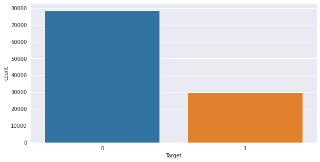
Univariate; analysis of one variable. Here we investigate trends per single column of interest. Keyword here is uni/one/single. We take a column of interest and investigate patterns in it before going to the next. For example we may want to know how the target variable in our sample dataset above is distributed, or the youngest and oldest customer and age group thresholds(definite age groups as seen in histogram bars). We do analysis column by column.

1
2
3
4

# Distribution of target variable
print(data.Target.value_counts())
plt.figure(figsize=(10,5))
sns.countplot(x=data.Target)

0    78735
1    29711
Name: Target, dtype: int64





<AxesSubplot:xlabel='Target', ylabel='count'>

1
2
3

# age into 6 groups
plt.figure(figsize=(10,5))
plt.hist(x=data.age, bins=6)

(array([30748., 30169., 22129., 17240.,  6919.,   919.]),
 array([15., 29., 43., 57., 71., 85., 99.]),
 <BarContainer object of 6 artists>)

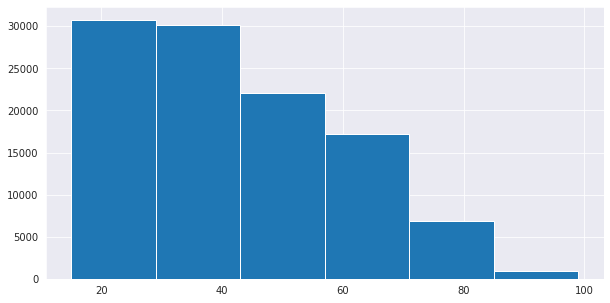
This information from the age column can be used to create a categorical variable as a feature engineering practice.

3. Bivariate Analysis

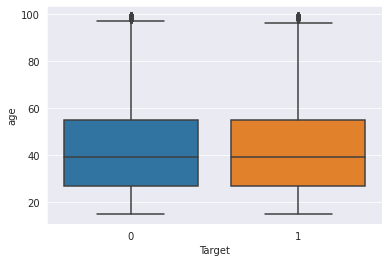
You guessed it! Here we do analysis of two variables. We try to determine the relationship between them. One type of plot that I never miss to use under bivariate analysis is the boxplot, especially in helping one to detect and remove outliers. It also helps one to visually see quartiles and their ranges.

1
2

# Boxplot
sns.boxplot(y='age', x='Target', data=data)

<AxesSubplot:xlabel='Target', ylabel='age'>

1
2
3

# Investigating correlation of country code and region
print(data[['country_code', 'region']].corr())
sns.heatmap(data[['country_code', 'region']].corr())

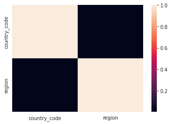
              country_code    region
country_code      1.000000  0.002045
region            0.002045  1.000000





<AxesSubplot:>

1
2

# Two variable regression joint plot
sns.jointplot(x='FQ28', y='FQ29', data=data, kind='reg')

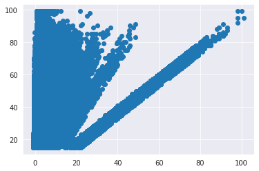
<seaborn.axisgrid.JointGrid at 0x7f48697e3400>

1
2
3

# add an imaginary continuous variable to show scatterplot between two variables
data['img'] = (data.age / data.country_code) + data.region
plt.scatter(x=data.img, y=data.age)

<matplotlib.collections.PathCollection at 0x7f48684f0370>

4. Multivariate Analysis

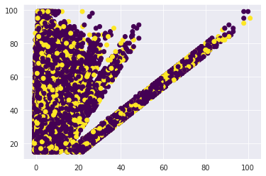
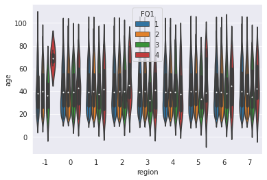
This involves observation and analysis of more than two variables at a time. We can also add onto bivariate analysis observations at this step by including the hue parameter to take care of a third distingushing feature between the two.

1
2

# Adding hue to the plot above
plt.scatter(x=data.img, y=data.age, c=data.Target, cmap='viridis')

<matplotlib.collections.PathCollection at 0x7f48681d6520>

1
2

# Observing variable quartiles separated by variable FQ1
sns.violinplot(x='region', y='age', hue='FQ1', data=data)

<AxesSubplot:xlabel='region', ylabel='age'>

To finish off multivariate analysis, there is one, many in one, plot that carries a lot of information from all the variables; the pairplot. For ease of readibility we’ll include only the first few columns together with the target variable since our dataset has a lot of variables:

1

sns.pairplot(data[list(data.columns[:10])+['Target']], hue='Target')

<seaborn.axisgrid.PairGrid at 0x7f4861c7c160>

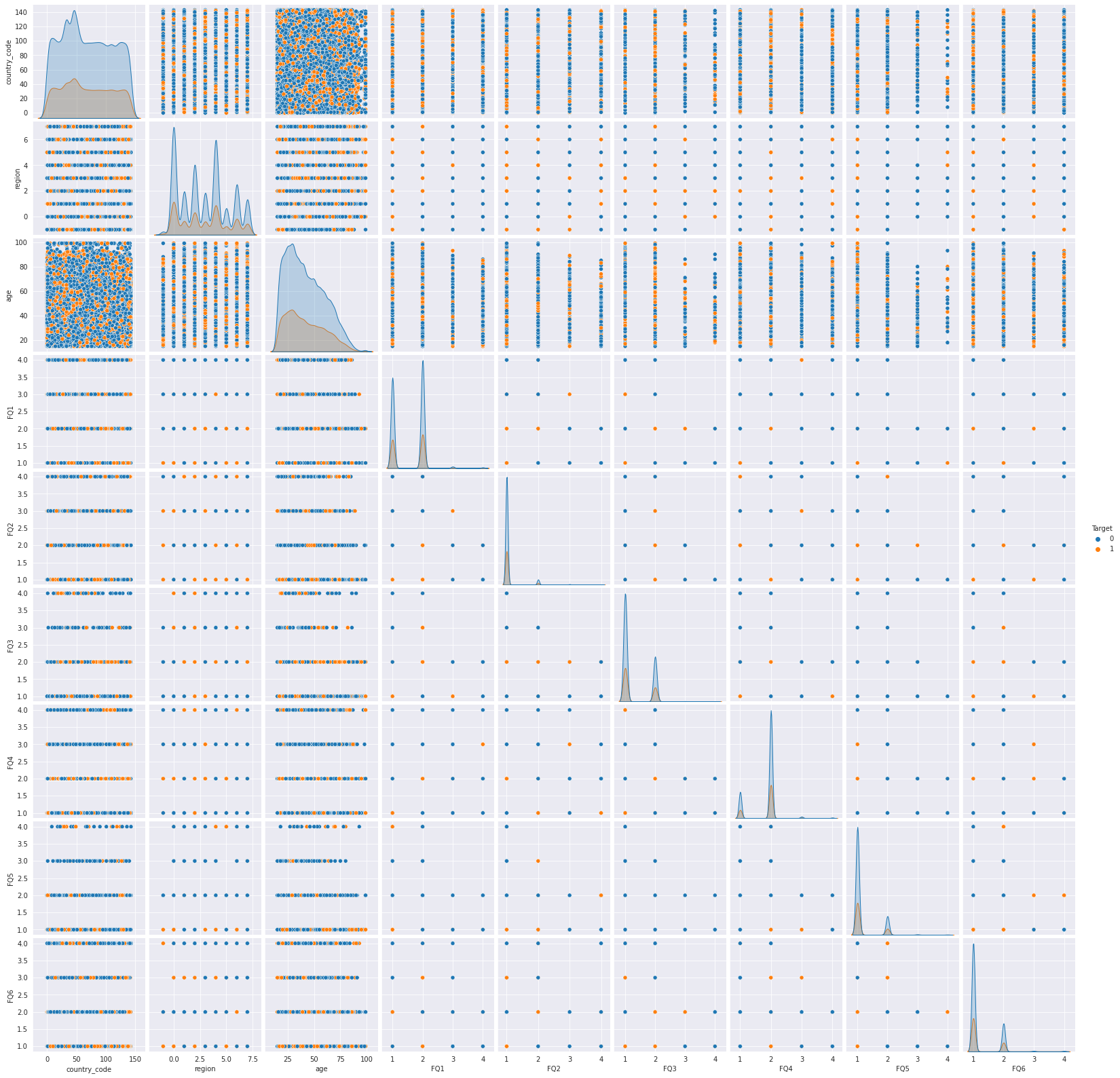
Most of the plots inside the pairplot don’t tell a lot of information in our case because these many variables are categorical. You should try it with a more receptive dataset.

These are the steps for exhaustive data analysis. We went through each giving a few examples. This guide does not cover everything, but it outlays a good procedure to follow for exhaustive EDA. It is good practice to go into details and make as many beatiful visualizations at each step, cheers!